


Anyone who's shopped at Amazon.com knows that you'll always end up buying more than you need. This is because Amazon uses a complex set of algorithms to recommend items based on what you're currently looking at. For example, if you're looking at a particular book on Steve Jobs, Amazon also recommends a list of other titles that other customers who bought this book also bought.).
Find additional: Artifical Intelligence Articles
Amazon does this by collecting data about what customers are buying, and using this huge set of data, it's able to make predictions about:
- Product trends and demands
- Inter-related products
- The reviews of products and their usefulness
The algorithms used by Amazon falls under the domain known as Machine Learning, sometimes also broadly known as Artificial Intelligence (AI).
Amazon isn't the only company using machine learning for its products. Uber, the ride-sharing giant, uses machine learning for all aspects of its operation. For example, it uses machine learning to:
- Provide you with an accurate estimate of when the car is going to show up when you request one
- Determine the correct pickup location based on your specified location
- Project the demands of customers and adjust its surge pricing
What's Machine Learning?
Machine Learning (ML) is a collection of algorithms and techniques used to design systems that learn from data. The algorithms of ML have a strong mathematical and statistical basis but they don't take into account domain knowledge. ML is comprised of the following disciplines:
- Scientific computing
- Mathematics
- Statistics
A good application of ML is trying to determine whether a particular credit card transaction is fraudulent. Given the client's past transaction records, it's the job of the data scientist to clean and transform it based on his domain knowledge so that he can apply the right ML algorithm to solve the problem (in this case, determine if a transaction is fraudulent). A data-scientist needs to know which method of ML will best help and how to apply it. He doesn't necessarily need to know how that method works, although knowing that will always help him to build a more accurate learning model.
What is Microsoft Azure Machine Learning Studio?
Microsoft Azure Machine Learning Studio (henceforth referred to as MAML) is an online, collaborative, drag-and-drop tool for building ML models. Instead of using the ML algorithms in languages like Python or R, MAML encapsulates most commonly used ML algorithms as modules and allows you to build learning models graphically using your dataset. This shields the beginning data science practitioners from the details of the algorithms, while at the same time offering the ability to fine-tune the hyper-parameters of the algorithm for advanced users. Once the learning model is tested and evaluated, you can publish your learning models as Web services so that your custom apps or BI tools, such as Excel, can consume it. What's more, MAML supports embedding your Python or R script within your learning models, giving advanced users the opportunity to write custom ML algorithms.
An Example: The Titanic Experiment
Now that you have a good sense of what ML is and what it can do, let's get started with an experiment using MAML before I discuss all the technologies and nitty-gritty behind ML. For this experiment, I'm going to use a classic example in ML - predicting the survival of a passenger on the Titanic.
In case you're not familiar with the Titanic, on April 15, 1912, during her maiden voyage, the Titanic sank after colliding with an iceberg, killing 1502 out of 2224 passengers and crew. The massive ship had been touted as unsinkable.
The main reason for the deaths was an insufficient number of lifeboats. Of those who survived, most were women, children, and members of the upper-class. This presents a very interesting experiment in ML. If we're given a set of data points containing the various profiles of passengers (such as gender, cabin class, and age, etc.) and whether they survived the sinking, it would be interesting to use ML to predict the survivability of a passenger based on his/her profile.
Interestingly, you can get the Titanic data from Kaggle (https://www.kaggle.com/c/titanic/data).
Kaggle is a platform for predictive modeling and analytic competitions in which companies and researchers post data, and statisticians and data miners compete to produce the best models for predicting and describing the data.
Two sets of data are provided:
- Training set
- Testing set
You use the training set to train your learning model to make predictions. Once your learning model is trained, you make use of the testing set to check the accuracy of your prediction.
Once the training and testing sets are downloaded, examine the content. Both (saved as CSV files) should have the following fields:
- PassengerId: a running number indicating the row of records
- Survived: whether the particular passenger survived the sinking
- Pclass: the ticket class the passenger holds
- Name: name of the passenger
- Sex: the gender of the passenger
- Age: the age of the passenger
- SibSp: number of siblings/spouses aboard the Titanic
- Parch: number of parents/children aboard the Titanic
- Ticket: ticket number
- Fare: the fare paid by the passenger
- Cabin: the cabin number
- Embarked: place of embarkation; note that C = Cherbourg, Q = Queenstown, S = Southampton
Using Microsoft Azure Machine Learning Studio
You're now ready to load the data into MAML. Using your Web browser, navigate to http://studio.azureml.net, and click on the Sign Up Here link.
If you just want to experience MAML without any financial commitment, choose the Free Workspace option and click Sign in. Other options include a free eight-hour trial and $9.99 a month for a subscription.
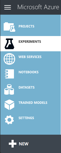
Once you're signed in, you see a list of items on the left side of the page (see Figure 1). I'll highlight some of the items on this panel as I go along.
Uploading Your Dataset
To create learning models, you need datasets. For this example, you'll use the dataset that you just downloaded.
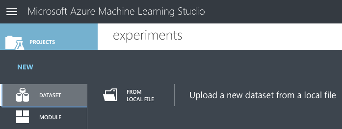
Click on the + NEW item located at the bottom left of the page. Select DATASET on the left (see Figure 2) and then click on the item on the right labeled FROM LOCAL FILE.
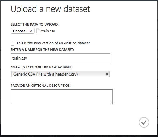
Click on the Choose File button (see Figure 3) and locate the training set downloaded earlier. When done, click the tick button to upload the dataset to the MAML.
Repeat the above steps to upload the testing dataset as well.
Creating an Experiment
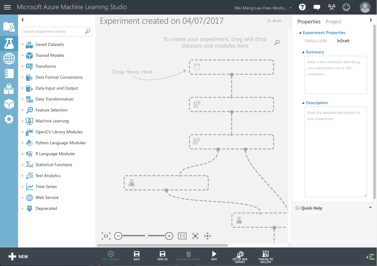
You're now ready to create a learning experiment in MAML. Click on the + NEW button at the bottom left of the page and select Blank Experiment.
You should now see the canvas shown in Figure 4.
You can give a name to your experiment by typing it over the default experiment name at the top. I chose Titanic Experiment.
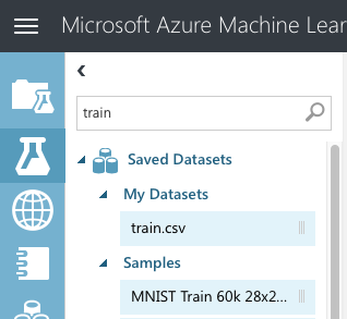
Once that's done, let's add the training dataset to the canvas. Type the name of the training set in the search box on the left and the matching dataset appears.
Drag and drop the train.csv dataset onto the canvas (see Figure 5).
The train.csv dataset has an output port (represented by a circle with a 1 inside). Clicking on it reveals a context menu (see Figure 6).
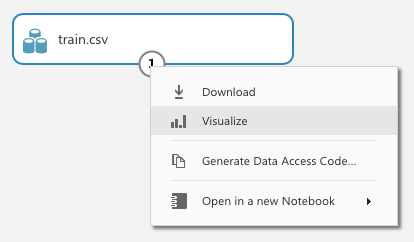
Click on Visualize to view the content of the dataset. The dataset is now displayed, as shown in Figure 7.
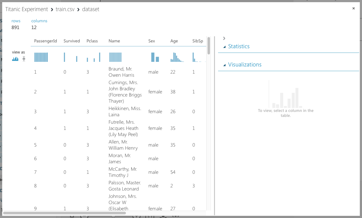
Take a minute to scroll through the data. Observe the following:
- The PassengerID field is merely a running number and doesn't provide any information with regard to the individual passengers. This field should be discarded when training your learning model.
- The Ticket field contains the ticket number of the passengers. In this case, a lot of these numbers seem to be randomly generated so it's not very useful in helping predict the survivability of a passenger. It should be discarded.
- The Cabin field contains a lot of missing data. Fields that have a lot of missing data do not provide insights to the learning model and should be discarded.
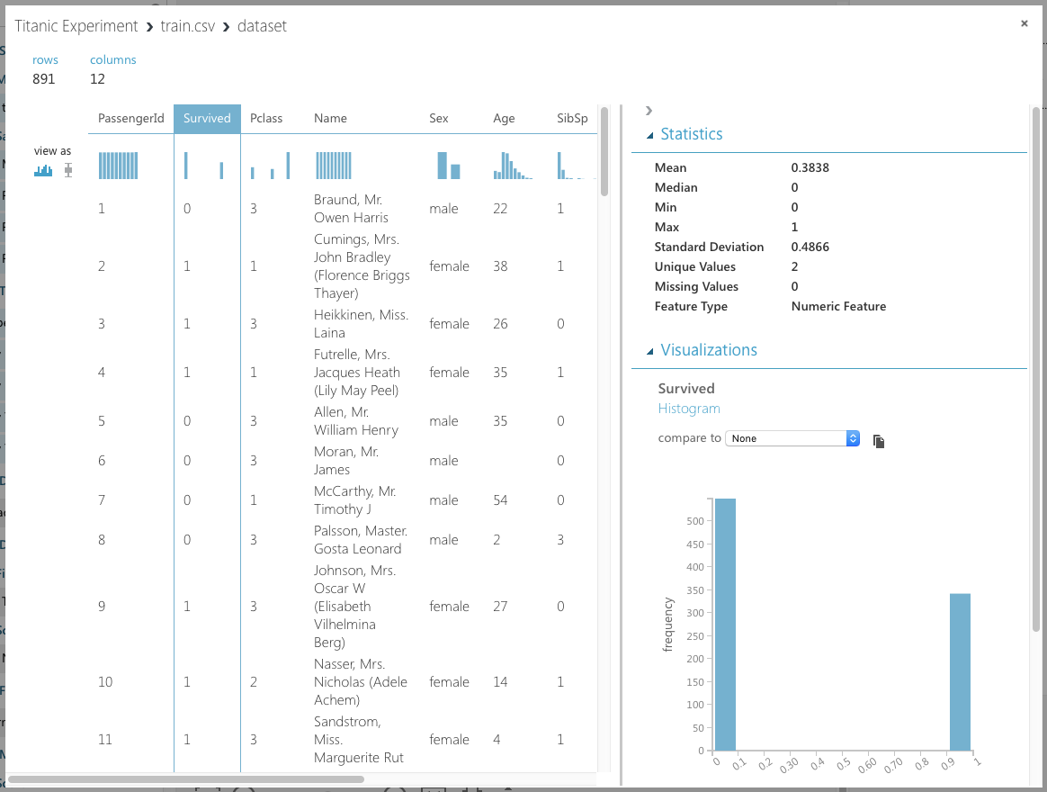
- If you select the Survived field, you'll see the chart displayed on the bottom right of the window (see Figure 8). Because a passenger can either survive (represented by a 1) or die (represented by a 0), it doesn't make sense to have any values in between. However, because it's represented as a numeric value, MAML won't be able to figure this out unless you tell it. To fix this, you need to make this value a categorical value. A categorical value is a value that can take on one of a limited, and usually fixed, number of possible values.
- The Pclass, SibSp, and Parch fields should all be made categorical as well.
All of the fields that aren't discarded are useful in helping create a learning model. These fields are known as features.
Filtering the Data and Making Fields Categorical
Now that you've identified the features you want, let's add the Select Columns in Dataset module to the canvas (see Figure 9).
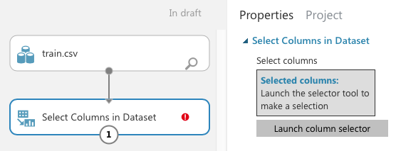
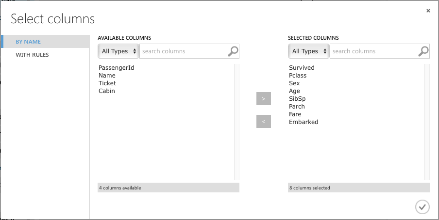
In the Properties pane, click on Launch column selector and select the columns, as shown in Figure 10.
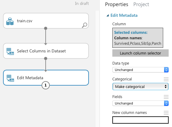
The Select Columns in Dataset module reduces the dataset to the columns that you've specified. Next, you want to make some of the columns categorical. To do that, add the Edit Metadata module as shown in Figure 11 and connect it as shown. Click on the Launch column selector button and select the Survived, Pclass, SibSp, and Parch fields. In the Categorical section of the properties pane, select Make categorical.
You can now run the experiment by clicking on the RUN button located at the bottom of the MAML. Once the experiment is run, click on the output port of the Edit Metadata module and select Visualize. Examine the dataset displayed.
Removing the Missing Data
If you observe the dataset returned by the Edit Metadata module carefully, you'll see that the age column has some missing values. It's always good to remove all those rows that have missing values so that those missing values won't affect the effectiveness of the learning model. To do that, add a Clean Missing Data module to the canvas and connect it, as shown in Figure 12. In the properties pane, select the Age column and set the Cleaning mode to Remove entire row.
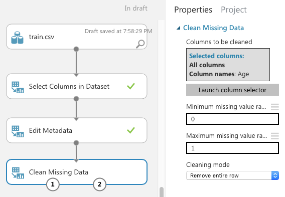
Click RUN. The dataset should now have no missing values. Also, observe that the number of rows has been reduced to 712.
Splitting the Data for Training and Testing
When building your learning model, it's essential that you test it with sample data after the training is done. If you only have one single set of data, you can split it into two parts: one for training and one for testing. This is accomplished by the Split Data module (see Figure 13). For this example, I'm splitting 80% of the dataset for training and the remaining 20% for testing.
For the case of the Titanic, you can always use the train.csv for training and test.csv for testing. For this example, I'm using the Split Data module to split the training dataset into two parts: one for training and one for testing.
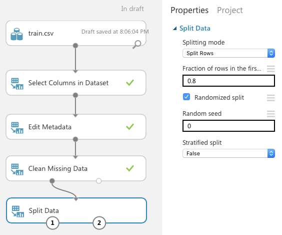
The left output port of the Split Data module provides the 80% of the dataset and the right output port provides the remaining 20%.
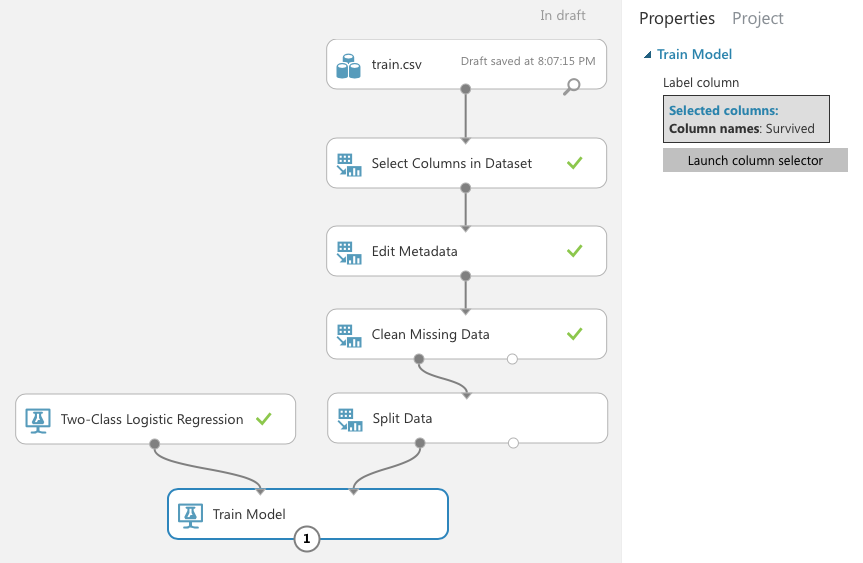
Creating the Training Model
You're now ready to create the training model. Add the Two-Class Logistic Regression and Train Model modules to the canvas and connect them, as shown in Figure 14. The Train Model module takes in a learning algorithm and a training dataset. You also need to tell the Train Model the label that you're training it for. In this case, it's the Survived column.
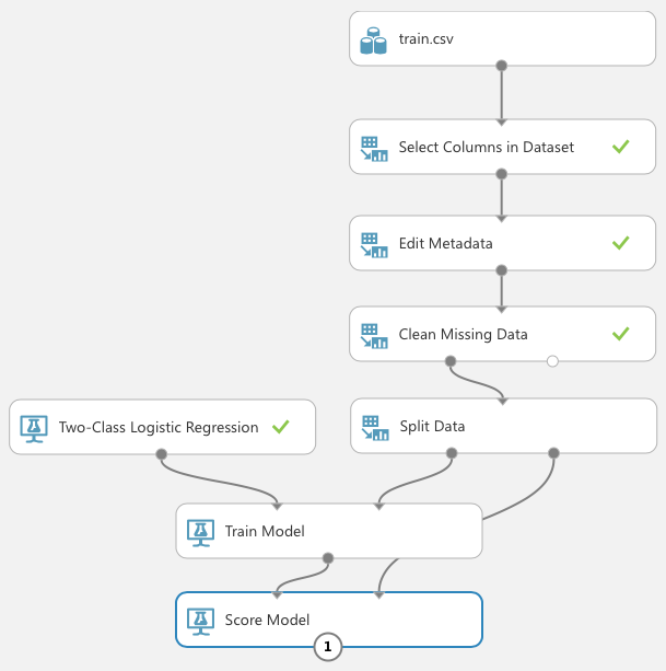
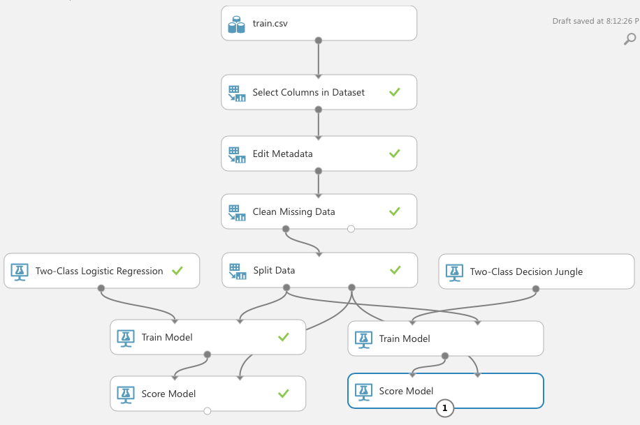
Once you've trained the model, it's essential that you verify its effectiveness. To do so, use the Score Model module, as shown in Figure 15. The Score Model takes in a trained model (which is the output of the Train Model module) and a testing dataset.
You're now ready to run the experiment again. Click RUN. Once it's completed, select the Scored Labels column (see Figure 16). This column represents the results of applying the test dataset against the learning model. The column next to it, Scored Probabilities, indicates the confidence of the prediction. With the Scored Labels column selected, look at the right-side of the screen and above the chart, select Survived for the item named compare to. This plots a chart known as the confusion matrix.
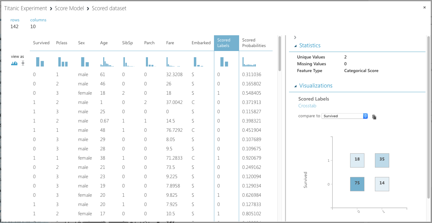
The y-axis of the confusion matrix shows the actual survival information of passengers: 1 for survived and 0 for died. The x-axis shows the prediction. As you can see, 75 were correctly predicted to die in the disaster, and 35 were correctly predicted to survive the disaster. The two other boxes show the predictions that were incorrect.
Comparing Against Other Algorithms
Although the numbers for the predictions look pretty decent, it isn't sufficient to conclude at this moment that you've chosen the right algorithm for this problem. MAML comes with 25 ML algorithms for different types of problems. And so, let's now use another algorithm provided by MAML to train another model: the Two-Class Decision Jungle.
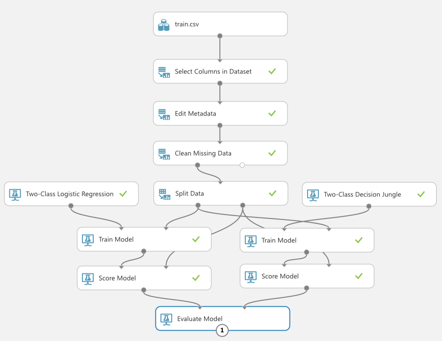
Add the modules, as shown in Figure 17.
Click RUN. You can click on the output port of the second Score Model module to view the result of the model, just like the previous learning model. However, it's more useful to compare them directly. You can accomplish this using the Evaluate Model module (see Figure 18).
Click RUN to run the experiment. When done, click the output port of the Evaluate Model module and you should see something like Figure 19.
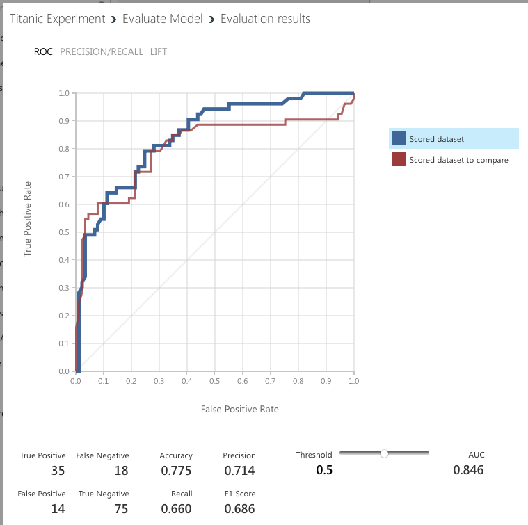
The blue colored line represents the algorithm on the left of the experiment (Two-Class Logistic Regression) and the red line represents the algorithm on the right (Two-Class Decision Jungle). When you click on either the blue or red box, you see the various metrics for each algorithm displayed below the chart.
Evaluating ML Algorithms
Now that you've seen an experiment performed using two specific ML algorithms, Two-Class Logistic Regression and Two-Class Decision Jungle, let's step back a little and examine the various metrics that were generated by the Evaluate Model module. Specifically, let's define the meaning of the following terms:
- True Positive (TP): The model correctly predicts the outcome as positive. In the case of the Titanic example, the number of TPs indicates the number of correct predictions that a passenger survived (a positive result) the disaster.
- True Negative (TN): The model correctly predicts the outcome as negative (did not survive). Passengers were correctly predicted to not survive the disaster.
- False Positive (FP): The model incorrectly predicted the outcome as positive, but the actual result is negative. In the Titanic example, it means that the passenger did not survive the disaster, but the model predicted the passenger to have survived.
- False Negative (FN): The model incorrectly predicted the outcome as negative, but the actual result is positive. Using the Titanic example, this means the model predicted that the passenger did not survive the disaster, but in actual fact, he did.
This set of numbers is known as the confusion matrix. Based on the above metrics, you can calculate the following metrics:
- Accuracy: This is defined to be the sum of all correct predictions divided by the total number of predictions, or mathematically, (TP/TN)/(TP+TN+FP+FN). This metric is easy to understand. After all, if the model correctly predicts 99 out 100 samples, the accuracy is 0.99, which would be very impressive in the real world. But consider the following situation: Imagine that you're trying to predict the failure of equipment based on the sample data. Out of 1000 samples, only three are defective. If you input a dumb algorithm that returns negative (meaning no failure) for all results, then the accuracy is 997/1000, which is 0.997. This is very impressive, but does this mean it's a good algorithm? No. If there are 500 defective items in the dataset of 1000 items, then the accuracy metric immediately indicates the flaw of the algorithm. In short, accuracy works best with evenly distributed data points, but works really badly for a skewed dataset.
- Precision: This metric is defined to be TP/(TP + FP). This metric is concerned with number of correct positive predictions. You can think of precision as “of those predicted to be positive, how many were actually predicted correctly?”
- Recall (also known as True Positive Rate): This metric is defined to be TP/(TP + FN). This metric is concerned with the number of correctly predicted positive events. You can think of recall as “of those positive events, how many were predicted correctly?”
- F1 Score: This metric is defined to be 2*(precision * recall)/(precision + recall). This is known as the harmonic mean of precision and recall and is a good way to summarize the evaluation of the algorithm in a single number.
- False Positive Rate (FPR): This metric is defined to be FP/(FP+TN). FPR corresponds to the proportion of negative data points that are mistakenly considered as positive, with respect to all negative data points. In other words, the higher FPR, the more negative data points you'll misclassify.
- To combine the FPR and the TPR into one single metric, you can first compute the two former metrics with different threshold (from 0.0 to 1.0), and then plot them on a single graph, with the FPR values on the x-axis and the TPR values on the y-axis. The resulting curve is known as the ROC (Receiver Operating Characteristic) curve, and the metric is considered the AUC (Area Under Curve) of this curve. In general, aim for the algorithm with the highest AUC.
The concept of precision and recall may not be apparent immediately, but if you consider the following scenario, it will be clear. Consider the case of breast cancer diagnosis. If a malignant growth is classified as positive and benign growth is classified as negative, then:
- If the precision or recall is high, it means that more patients with actual breast cancer are diagnosed correctly, which indicates that the algorithm is good.
- If the precision is low, it means that more patients without breast cancer are diagnosed as having breast cancer.
- If the recall is low, it means that more patients with breast cancer are diagnosed as not having breast cancer.
For the last two points, having a low recall is more serious than a low precision (although wrongfully diagnosed as having breast cancer when you do not have it will likely result in unnecessary treatment and mental anguish) because it causes the patient to miss treatment and potentially causes death. Hence, for cases like diagnosing breast cancer, it's important to consider the precision and recall metric when evaluating the effectiveness of an ML algorithm.
Publishing the Learning Model as a Web Service
Once the most effective ML algorithm has been determined, you can publish the learning model as a Web service. Doing so allows you to build custom apps to consume the service. Imagine that you're building a learning model to help doctors diagnose breast cancer. Publishing as a Web service allows you to build apps to pass the various features to the learning model to make the prediction. Best of all, using MAML, there's no need to handle the details of publishing the Web service; MAML hosts it for you on the Azure cloud.
Publishing the Experiment
To publish the experiment as a Web service:
- Select the left Train Model module (because it has a better performance compared to the other).
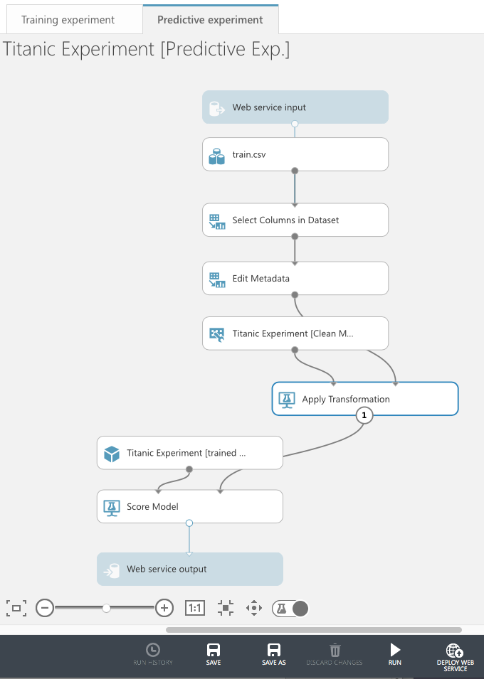
- At the bottom of the page, hover your mouse over the item named SET UP WEB SERVICE, and click Predictive Web Service (Recommended).
This creates a new Predictive experiment, as shown in Figure 20.
Click on RUN and then DEPLOY WEB SERVICE. The page depicted in Figure 21 is shown.
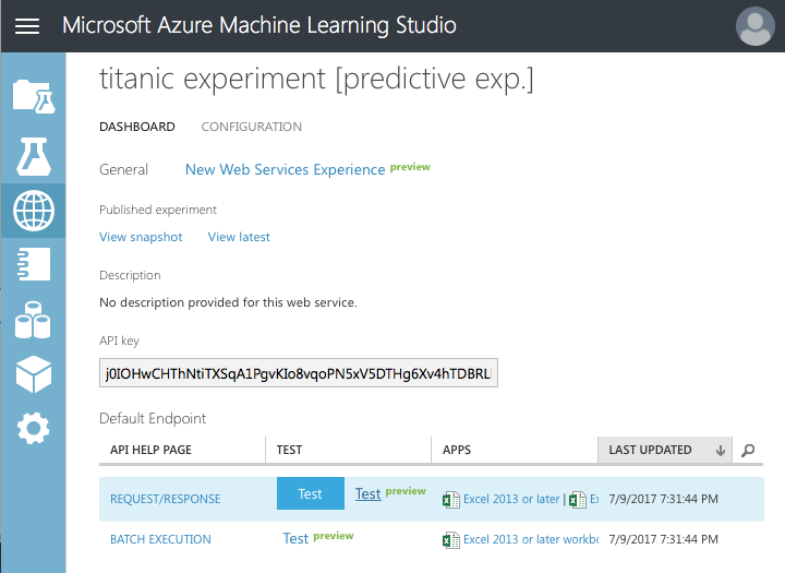
Testing the Web Service
Click on the Test hyperlink. The test page shown in Figure 22 is displayed. You can click on the Enable button to fill in the various fields from your training set. This saves you the chore of filling in the various fields.
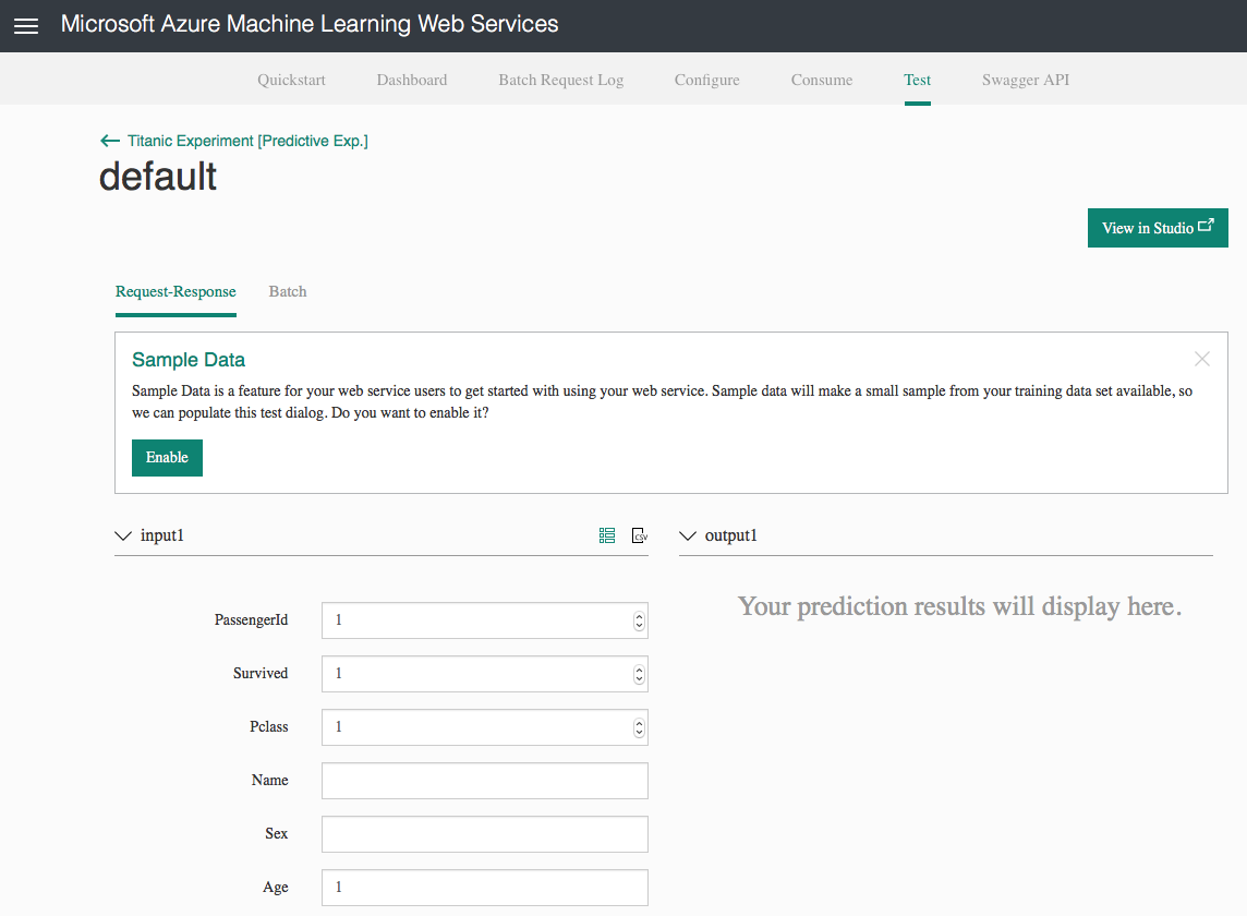
The fields should now be filled with values from the training data. At the bottom of the page, click Test Request/Response and the prediction will be shown on the right.
Programmatically Accessing the Web Service
At the top of the Test page, you see a Consume link. Click on it.
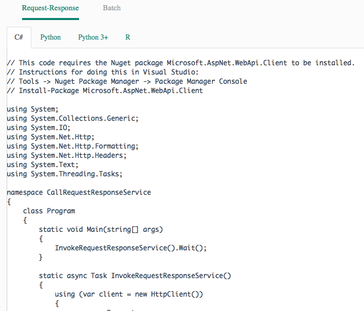
The credentials you need to use in order to access your Web service, as well as the URLs for the Web service are now visible. At the bottom of the page, you'll see the sample code generated for you that you could use to programmatically access the Web service (see Figure 23). The sample code is available in C#, Python 2, Python 3, and R.
Click on the Python 3+ tab and copy the code generated. Back in MAML, click on the + NEW button at the bottom of the screen. Click on NOTEBOOK on the left and you can see the various notebooks as shown in Figure 24.
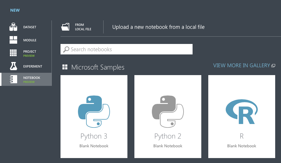
Click on Python 3, give a name to your notebook, and paste in the Python code that you copied earlier (see Figure 25).
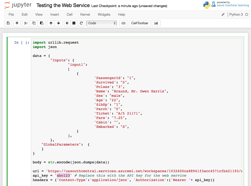
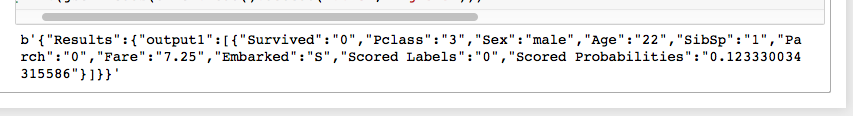
Be sure to replace the value of the api_key variable with that of your primary key. Press Ctrl+Enter to run the Python code. If the Web service is deployed correctly, you can see the result at the bottom of the screen (see Figure 26).
Summary
In this article, you've learned the basics of ML and how you can build a learning model using the Microsoft Azure Machine Learning Studio. With MAML, it's now very easy to start developing and testing your learning models without getting bogged down with the details of the learning algorithms. Happy ML!