


Imagine you're working for a company that has accumulated a tremendous amount of transaction data. The business users want to perform all sorts of analysis, monitoring and analytics on the data. Some OLTP developers might reply with, “Just create views or stored procedures to query all the data the way the users want.” Many companies initially take that approach - however, just like certain technologies and system hardware configurations don't scale well, certain methodologies don't scale well either. Fortunately, this is where data warehousing and dimensional modeling can help. In this article, I'll provide some basic information for developers on the basics of data warehousing and dimensional modeling - information that might help you if you want to provide even more value for your company.
Required Reading
This area of interest has many good books including the “desert island classics” like the famous Design Patterns: Elements of Reusable Object-Oriented Software by the Gang of Four, and the Refactoring: Improving the Design of Existing Code book by Martin Fowler. If you want to learn about data warehousing and dimensional modeling, then THE book to read is The Data Warehouse Toolkit: The Complete Guide to Dimensional Modeling, by Ralph Kimball. First, this is NOT a book on technology - it is a book about methodologies and repeatable patterns for assembling data based on business entities. Kimball wrote the book in 2004, and the book is just as relevant today as it was almost a decade ago.
This article will introduce many of the concepts that Kimball covers. I'm going to keep the examples very basic and fundamental. I strongly recommend you check out the Kimball website: https://www.kimballgroup.com/. You'll find many categories on the website, including an excellent section of design tips: https://www.kimballgroup.com/category/design-tips/
(Note that I'm not formally associated with Kimball or the Kimball Group in any way. I've implemented his methodologies in work projects and I - along with countless other developers - have benefited from his efforts).
What's on the Menu?
Here are the topics for this article:
- Major components of a data warehouse
- Cumulative transactional fact tables
- Factless fact tables
- Periodic snapshot fact tables
- General contents of dimension tables
- Snowflake dimension schemas
- Role-playing dimensions
- Junk dimensions
- Many-to-many dimension relationships
- Type 2 Slowly Changing Dimensions (SCD)
- A word about storing NULL foreign keys in fact tables - DON'T!
- Conformed (common) dimensions
- What (not) to store in fact tables
Tip 1: Major Components of a Data Warehouse
While you can walk into ten different companies and see up to ten different database topologies, a very common challenge that project managers face is integrating data from multiple data sources. Whether a database team needs to integrate shipment, spending, budget, and retail data - or needs to integrate patient demographic, diagnosis, claims, and billing data - there will always be the need to cleverly combine data from different sources to produce one clean version of “the historical truth.”
The need arises (in part) from the fact that nearly every organization has a value chain - a progression (chain) of related activities associated with a company's business processes. In most of the activities, data is collected, though the collection process might span many disparate systems, with data collected at different levels of granularity, time periods, etc. A goal of data warehousing is to bring all of the data “under one umbrella,” after a series of validations, grouping, splitting and any other forms of synthesis.
Figure 1 shows a diagram that many have probably seen at some point in their careers: a high-level process flow that begins with multiple data sources (often from transactional systems) and ends with a data warehouse (comprised of a set of data marts that might be used to create OLAP cubes for more advanced analytic purposes).
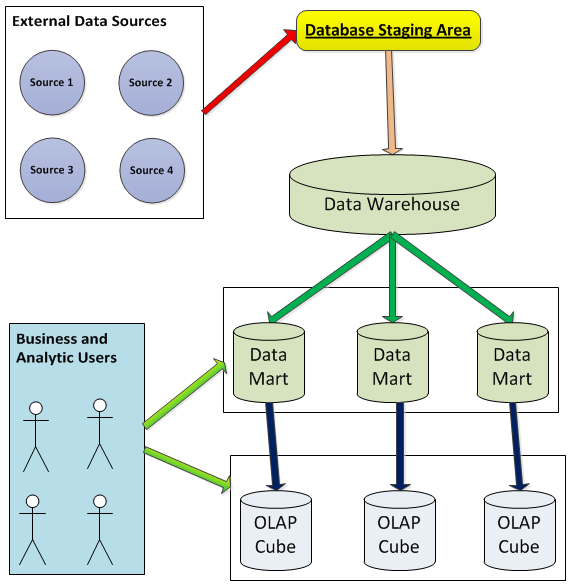
Note that developers will rarely transfer data directly from the original OLTP sources to the data warehouse - usually developers will load data into a temporary staging area (on an overnight basis, weekly, etc.) and perform validations or possibly “re-shape” the data before eventually pumping the data into the data warehouse/data marts.
One of the signature characteristics of most data warehouses is that the data is structured into fact and dimension tables. Fact tables contain the business measures (metrics), which can be anything from revenue to costs to premium payment amounts. Dimension tables provide business context to the fact tables, which can be anything from products to customers to cost centers, etc. Ultimately, business users evaluate the measures “by” the different related business dimensions.
These fact and dimension tables are usually organized in a de-normalized (star-schema) form. This is often culture shock to long-term OLTP developers who are used to databases in third-normal form. The thing to remember is that normalization is necessary to save data as efficiently as possible. In a data warehouse, the goal is to retrieve data as efficiently as possible.
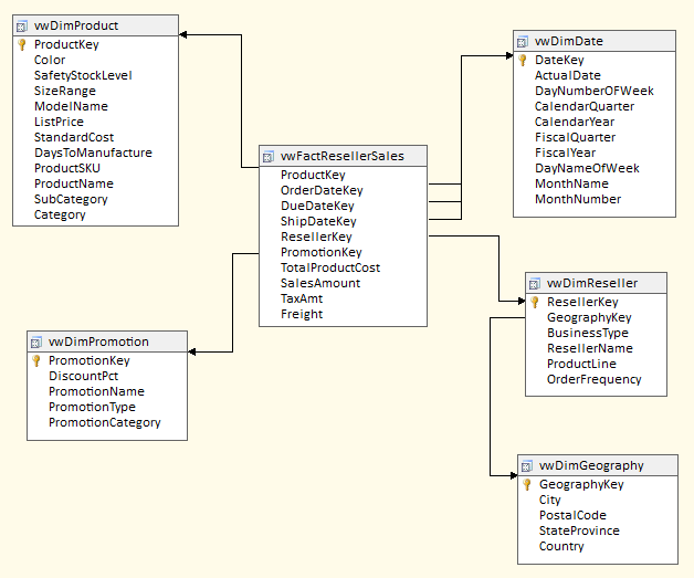
Figure 2 shows a simple but meaningful star-schema, fact-dimension model using some of the AdventureWorks data. The fact and dimension tables are usually related through surrogate integer keys. The dimension tables contain primary keys for each business entity value, along with a business key and all of the attributes that further describe the entity value (for instance, a specific product has a SKU number, a color, a list price, and belongs to a particular subcategory, category, brand, etc.). The fact tables contain foreign key references to the dimension values, along with the measures. End users often will “roll up” the measures by any related dimension attribute.
Tip 2: Cumulative Transactional Fact Tables
Tip #1 provided an overview for a data warehouse and a small example of a fact/dimension table scenario. It should be no surprise that there are many specific topics and therefore many “stories” surrounding data warehouse models. The next several tips will look at some of these topics.
First, fact tables generally fall into one of two categories - they are either “cumulative transaction” or “snapshot” fact tables. I'll talk about cumulative transaction fact tables in this tip and in Tip #3. I'll talk about snapshot fact tables in Tip #4.
Cumulative transaction fact tables are those where business users can fully aggregate the measures by any related dimension, usually without limitation. An example would be a fact order table, with measures for order amount, cost, freight, discount, etc. If 10,000 new orders are placed daily, the processes that populate the data warehouse will insert the new orders into the fact order table. We generally refer to these measures as “fully aggregatable.”
Tip 3: Factless Fact Tables
Before I move on to the second type of fact table (periodic snapshot fact table), I want to talk about a special type of cumulative transactional fact table called a “factless fact table.” This almost sounds like a contradiction in terms, but here is a scenario to help explain.
Suppose you have a need to track the tally of students who register for classes over time. You might want to aggregate (count) the number of students by time period, by class, by major, by instructor, etc.
The fact table might not contain any actual measures - so it might not initially seem very glamorous or interesting. But what might be of interest to analysts is the number of times where dimensions come together to “form an event” - whether it is enrollment in a class or attendance in a class for a day. Other examples might include the number of times a product is promoted in certain cities across certain time periods.
In all cases, the factless fact table might only contain dimension foreign keys, where the application software/query will count and group by the desired dimension attributes. (In some instances, there will be a numeric column with a value of 1 or 0 for a single measure, and the query will sum that numeric column.)
So again, while not as glamorous as a fact table that rolls up to millions of dollars, factless tables can be very important for an analyst who need to see tallies over time when dimensions came together to form some business event “in the value chain.” (Do you see how these things are starting to come together?)
Tip 4: Periodic Snapshot Fact Tables
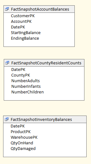
Just about everyone has some type of checking/banking account. Most banks produce some type of statement that lists (among other things) the starting and ending balance for each period (month). Suppose the bank generated a fact table of monthly balances by customer and month. I might have a month-ending balance of $1,000 in January of 2013 and a month-ending balance of $1,500 in February of 2013. Unlike the cumulative transactional fact table (where measures are fully additive and aggregatable), I wouldn't want to sum the ending balance for my account across all of time - the value of $2,500 would not make any analytic sense. The two distinct values of $1,000 and $1,500 were not meant to be summarized - they represented two “snapshots” of a metric based on a specific point in time. An analyst might summarize the balances across all customers for one time period, or even average the balances for a single customer across all time periods - but the point is that restrictions are necessary on any aggregations.
Another example is inventory counts - we might conduct a basic inventory of product shelf counts by month. In January we might have a quantity of five for a specific product SKU, and a quantity of four the next month. We would not sum the number across time periods, because that was not the intention of the original number. Again, we might perform an average, or restrict how we sum - but the point is that the measures can only be partly rolled up - or as some would say, the measures are “partially additive.”
In a prior lifetime, I worked in WIC and I worked in Medicaid. Both were invaluable experiences in the world of data. One of the many requirements in both areas was a monthly count of participants in the program by different business entities (by infants and children and by county and health assessment….or by Medicaid provider/facility and utilization group, etc.) With any participation program, you will have some people enter the program one month and drop off in a few months - so any tally or summarization of measures needs to be restricted to certain periodic intervals. Otherwise, the same person would be counted twice if an aggregation occurs across months, which wouldn't make any sense.
These are three business scenarios where we need to store tallies, counts, or other statistics that represent a point-in-time snapshot (which could be a month, quarter, etc.). The numbers are not cumulative, and therefore would not be rolled up across all measures. We call these types of fact tables “periodic snapshot” fact tables, which are often populated by some end of period process, and are only intended to be aggregated in limited ways (partially additive). It is not unusual for a data warehouse to have (for example) six transactional fact tables and one or two periodic snapshot fact tables.
With both transactional fact tables and periodic snapshot fact tables, we generally insert into these tables, and only perform updates based on corrections. However, in some scenarios (often with accounting implications), data is NEVER modified in data warehouse fact tables: in that situation, corrections are handled by reversing entry rows.
There is only one exception, where a fact table might be updated as a normal sequence of events - this is a variation of a snapshot fact table called an “accumulating snapshot fact table,” where columns of a row are updated to reflect the business process of the row. An example might be a mortgage application row, with separate columns for approval dates and approval amounts. This is not a common type of fact table, and some database architects prefer to normalize the fact table and generate separate rows for each phase/milestone.
I've included some examples of snapshot fact tables in Figure 3.
Tip 5: General Contents of Dimension Tables
Back in Figure 2, I included an example of a product dimension. Other examples of dimension tables could be anything from date calendar, service, geography, general ledger, merchandising type, vendor, etc. They represent the different business entities by which users wish to analyze measures.
Dimensions normally contain the following sets of columns:
- A single integer surrogate key.
- A single business key (used during ETL processes to match up rows, since external applications will reference the business key and not the surrogate key).
- Typically one or more description columns (maybe a short description for application dropdowns that need to show a narrow description, and a longer description for report output where wider descriptions can be used).
- Attributes that form a parent-child hierarchy (for instance, subcategory->category->brand).
- Attributes that have no relationship to each other (list price, color, weight, etc.). One thing to remember here: suppose you have 1,000 products with 900 distinct list prices. Business analysts might choose to group the list prices into a shorter, more discrete (and more manageable) range of list prices. Unless, of course, there is analytic value to summarizing sales by each and every one of the 900 list prices.
- In some instances, a column to define the sort order (for instance, products might be sorted neither by description nor by SKU number, but by some custom order reflected in a single integer column).
In general, all the attributes (columns) of a business dimension should reflect those characteristics that describe the row, and should reflect those areas by which users want to aggregate and “slice and dice” historical fact table data.
A final word on business dimensions: while the dimensions can vary tremendously across companies, the one dimension that is almost universal is a date dimension. It is almost inconceivable that a data warehouse would not have a dimension to evaluate measures over time. Some date dimensions might be very simple, with attributes for date, month, and year. Other date dimensions might be more complex, with the following sets of attributes:
- Week-ending dates (e.g. for Sunday to Saturday ranges)
- Regular calendar month/quarters and Fiscal month/quarters
- Week or period numbers
- Attributes for seasonality (i.e., events whose dates vary across years, such as Lent weeks, Black Friday, etc.)
Tip 6: Snowflake Dimension Schemas
While many data warehouse professionals prefer the simplicity and elegance of denormalized star schemas, sometimes “snowflake” dimension schemas are needed. Snowflake schemas are ones where dimensions are spread out in a more normalized manner. Here are two scenarios where snowflake schemas might be called for:
- When you have multiple fact tables at different levels of granularity. For example, you might have revenue at the product SKU level and budget/forecast data at the product brand level. In that case, you might create a “mini-dimension” of product brands that conforms to the brands in the lower level product dimension.
- If you have parent/child attributes in a dimension, and the parent attribute has a large number of properties. For instance, I might be one of thousands of residents who lives in a county. The county might have a very large number of demographic attributes at the county level. Rather than repeat a large number of attributes in the resident dimension (where there would be relatively little variance across residents), we might create a special type of normalized county dimension called a “dimension outrigger” where the attributes are stored in the parent dimension. Ralph Kimball talks about dimension outriggers as a notable exception to the goal of building star-schema models.
Tip 7: Role-playing Dimensions
Suppose you have a fact table of orders, with three different dates for each order - original order date, ship date and delivery date. Depending on the type of business, the lag across the three dates could be a few days or longer.
A business might want to roll up order dollars (or some other measure in the fact table) by month based on the original order date (when the order dollars were booked). However, they might also want to roll up a measure in the order table based on delivery month.
Figure 4 shows an example where a single date dimension key might be used in multiple PK/FK relationships into a fact table. We call this a “role-playing” relationship because the date key is servicing multiple purposes (or “roles”) into the fact table.
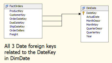
Dates are the most common scenario with role-playing dimensions. Another example could be an airport dimension associated with multiple foreign keys in a flight fact table, one for expected flight destination airport code and one for the actual flight destination airport code. (I'm sure at least one reader has attempted to fly to Fargo and landed in Minneapolis instead!)
Tip 8: Junk Dimensions
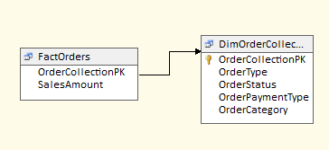
Some fact tables might be related to multiple dimension tables that each contain a small number of rows. For instance, in Figure 5, we have an order table with links to order type, payment, status and category dimensions. While there's nothing wrong with this, another pattern that might server better is a “junk dimension” that holds a Cartesian product of every possible type, payment, status and category value in a single dimension, with a surrogate identifier that is stored in the fact table (Figure 6).
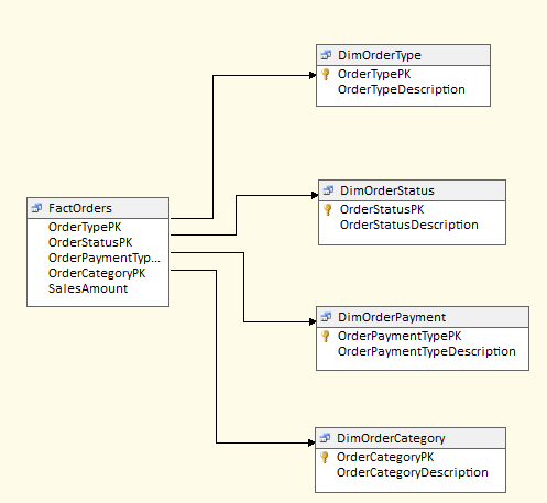
The end user will still be able to “slice and dice” and aggregate order measures by any or all of the four attributes - while the number of dimensions is simplified. There is no set rule for the maximum number of rows that will still effectively represent a junk dimension - though this approach is typically for status and other indicators and enumerations that generally have a handful or perhaps a few dozen values. So while not the most mission-critical dimension modeling pattern, it can add a small level of simplicity to an otherwise larger and more unwieldy number of dimensions.
Tip 9: Many-to-Many Dimension Relationships
In some scenarios a “bridge table” is necessary to associate facts with dimensions. Here are some scenarios:
- Suppose you have a fact table of sales for computer books. A book can be written by multiple authors, and a single author can write multiple books. You might want to break out sales by author, factoring in the author's percentage of contribution towards the book. The fact table of sales might only contain the book PK, but no author PK. A bridge table containing each author/book combination (and the author's percentage of contribution) might be necessary.
- Suppose you have product shipments expressed in terms of lbs, but you might want to express volume shipped in terms of other volumetrics (cases, retail units, etc.). You might need a bridge table that contains each product, unit of measure, and a conversion factor with respect to the base UOM (lbs).
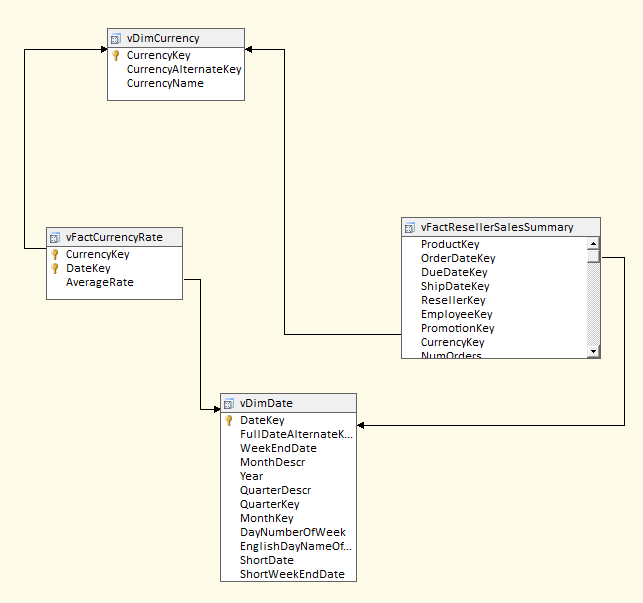
- In the case of the AdventureWorks sample database, suppose you have sales dollars expressed in terms of the U.S. dollar, but you want to display sales in terms of other currencies, knowing that a bridge table of currencies and exchange rates by day will be necessary.
All three of these bridge (many-to-many) table scenarios seem like very different scenarios - but they all share a common pattern. In all cases, we want to aggregate a fact table by a business entity that is not associated with the fact table (authors, units of measure, currency) - but where the entity “is” associated with another entity (books, products, dates) that IS directly tied to the fact table.
Figure 7 shows an example of a bridge table for the third relationship (involving currencies).
Tip 10: Type 2 Slowly Changing Dimensions
One of the more critical aspects of data warehousing can be accounting for Type 2 Slowly Changing Dimensions (also known as SCD). Here is a scenario:
Suppose a product goes through three price changes over the course of two years. You want to track the history of sales (and returns) when the product was under each price. We refer to this as a Type 2 Slowly Changing Dimension, where we want to preserve history. (By contrast, in a Type 1 Slowly Changing Dimension, we simply overwrite the price attribute in the dimension and we don't care about history.)
Implementing a Type 2 SCD means accounting for the following (reflected in Figure 8):
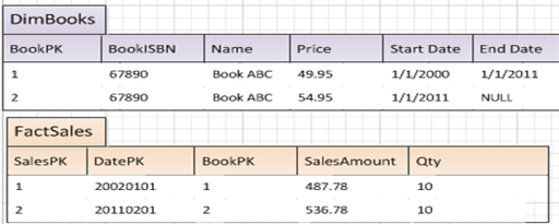
- The dimension (in this case, product dimension) should contain startDate/enddate columns for the time period when the state of the row (product) is in effect.
- When an ETL process detects a product price change, the ETL should “retire” the old version of the row (based on the business key, the Product SKU) by marking the end date, and then insert the new version of the row (same Product SKU, but different surrogate key) and a new start date.
- When the ETL process writes out new sales rows, the process should look for the product surrogate dimension key that represents the version of the product that was “in effect” at the time of the sale. This is why the product dimension needs to have startdate/enddate columns.
Tip 11: A Word about Storing NULL Foreign Keys in Fact Tables - DON'T!
In most disciplines, there are (as an old boss used to say to me) “blue rules” and “red rules.” The blue rules are general guidelines for most scenarios, but might need to be bent in certain situations. Red rules are ones you never ever violate.
Here's a red rule, one you should never violate. Never store NULL values in a fact table foreign key. Here's a scenario - suppose you have a fact table of orders by product, customer, date and cost center. On 95% of the orders, there is a valid cost center - but on 5% of the orders, there is no cost center. (Maybe it's an irregular or internal order, etc.). Some database people (often those who have only worked in OLTP environments) will want to store a NULL value in the cost center foreign key. While SQL Server (and other databases) will permit this (assuming the column is NULLable to begin with), in practice this is a terrible idea.
Why is it terrible? Because it makes it very difficult for business users to analyze order dollars aggregated by cost center and also include orders where no cost center existed. The recommended practice is to store a “dummy row” in the cost center master dimension (something like “Unused or Undefined Cost Center”) and then utilize the surrogate key for that row when writing to the fact table. This will help end users greatly when they need to do exception reporting. Some of the most intense disagreements I've had have been with people who wanted to store a NULL value in the fact table. Again, this is a very bad idea!
Tip 12: Conformed (Common) Dimensions
One of the many reasons I love the data warehousing industry is that there are so many recommended practices and patterns to guide the dimension modeling process. The Kimball methodology provides many good rules, some of which I've talked about already. Another good one is the concept of conformed dimensions. As I describe this topic, you might say to yourself, “Well, yeah….of course, that's just common sense.” But of course, anyone who has seen client databases knows that common sense is not always practiced!
Suppose you have multiple data marts that make up a full data warehouse. A product dimension might be a common dimension across the data marts (and across the value chain in the company). The concept of conformed dimensions means that if a product key is used as the level of granularity across many fact tables in many data marts, that product key must have the exact same context in each data mart. One data mart might have sales through one sales channel, and a second data mart might have sales through a different sales channel. If someone wants to analyze sales by product across the two channels, the context of each product key must be identical across the two data marts. This is what is known as a common/conformed dimension.
Again, you might read this and say, “Right….how could it be anything other than that?” And that's the correct way to approach the situation!
Tip 13: What (Not) to Store in Fact Tables
Sometimes fact tables might contain calculated measures derived from other measures. This is fine for simple calculations where the measure is still additive. For instance, a fact table might contain measures for gross revenue and returns, and then a third physical measure for adjusted revenue (as gross revenue, less returns). While some might debate that the physical measure takes up disk space and could be calculated, there's nothing analytically wrong with the calculation.
However, creating measures from calculations involving division is a different story. Suppose you had two stores. One store had 10 dollars in returns and 20 dollars in sales - the returns rate as a % of sales would be 50%. The second store also had 10 dollars in returns and 100 dollars in sales - the returns % for the second store would be 10%. If you stored both percentages in a returns % column, how would you aggregate the % if someone wanted the total returns % for the region? You certainly wouldn't add the two percentages together - and taking a straight average of the two wouldn't reflect the true weight of the two stores. The only correct methodology would be to sum the returns across all stores (20 dollars) and divide by the sum of sales across all stores (120 dollars), and then divide the sums (20/120, or 16.67%).
So the bottom line is this: you don't want to store calculations involving ratios or percentages in fact tables - instead, you want to store the numbers that represent the numerator and denominator of the calculation, and then calculate the % on the fly, based on whatever dimensions someone uses. Or, as Kimball states in his famous dimension modeling book, Percentages and ratios, such as gross margin, are non-additive. The numerator and denominator should be stored in the fact table. The ratio can be calculated in a data access tool for any slice of the fact table by remembering to calculate the ratio of the sums, not the sum of the ratios.
You don't want to store calculations involving ratios or percentages in fact tables - instead, you want to store the numbers that represent the numerator and denominator of the calculation, and then calculate the percentage on the fly depending on the context.
Last Call - Some Final Notes
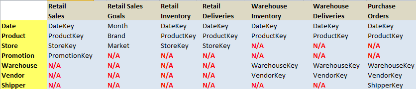
Here are some final random notes. First, I've tried to keep the examples here very basic and fundamental. Obviously, in actual applications, fact and dimension tables are likely to be more complicated. Developers will face many fact tables with partial commonality across dimensions, and also fact tables built at different levels of granularity. Kimball's dimension modeling book discusses fact/dimension table usage and relationships, and the need to establish a matrix of where fact tables intersect (and don't intersect) with dimension tables. Figure 9 shows an example that's very similar to one of the examples in his book: I've added a sales goal fact table into the mix to demonstrate that some sales fact data might be at the product and account and date level, while a sales goal table might be set at a much higher level.
Second, note that this article hasn't included any code (yes, I realize the name of this magazine is CODE Magazine!). Hopefully you've picked up a few tips you didn't know about building fact/dimensional models. Additionally, good T-SQL chops will always be necessary to shape data into fact/dimension structures. I've told developers and students for several years now that if they haven't learned the MERGE statement in T-SQL, that they should study it until their eyes are sore. MERGE has become a very popular feature in the data warehousing process. I've written about MERGE in different Baker's Dozen articles over the last year, and I definitely recommend you take a look at the feature. I also recommend that database developers learn SSIS. While some companies use all the data-handling features of SSIS and others use it more as a general workflow manager, SSIS is a powerful ETL tool that many companies use in building data warehouses.