


To use a music analogy, many installments of “The Baker’s Dozen” have been like “concept albums,” where most or all of the tips work towards a big picture. Then there are times where I present a series of random tips that are largely standalone and don’t form a pattern. In this article, I’m going to present 13 random tips for SQL Server and T-SQL programming.
What’s on the Menu?
Getting right to the point, here are the 13 items on the menu for this article:
- Baker’s Dozen Spotlight: A T-SQL tip for summarizing data by week, and calculating a 52-week moving average
- Using SQL Server table-valued functions as a means of implementing security access by business entities
- SQL Server covering indexes for performance
- SQL Server SARGs (Searchable Arguments)
- T-SQL SUM OVER capability to implement a % of Parent calculation
- Programmatically disabling SQL Server constraints and triggers
- Correlated subqueries and derived table subqueries and their execution plans
- A little brain teaser on the UNION statement
- Back to basics - determining when a subquery is necessary
- The tinyint data type and when to use it
- DISTINCT vs GROUP BY
- Creating a result set of integers for a picklist
- INSTEAD OF triggers to prevent deletions
The Demo Database for the Examples
With just a few exceptions, the examples use the AdventureWorks2008R2 database. You can find AdventureWorks2008R2 on the CodePlex site. If you’re still using SQL Server 2008 and not 2008R2, the examples will still work - you’ll just need to change any 2008R2 references to 2008.
Tip 1: Baker’s Dozen Spotlight: Summarizing Data by Week and Calculating a 52-week Moving Average
Scenario: I want to take daily sales information from the daily Purchase Order table in the AdventureWorks database and summarize sales by week ending date. For each week, I also want to calculate the average weekly sales going back over the last 52 weeks.
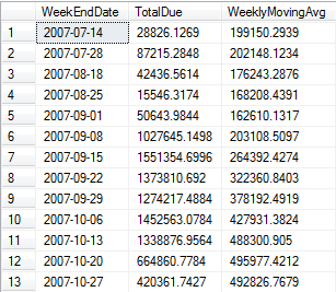
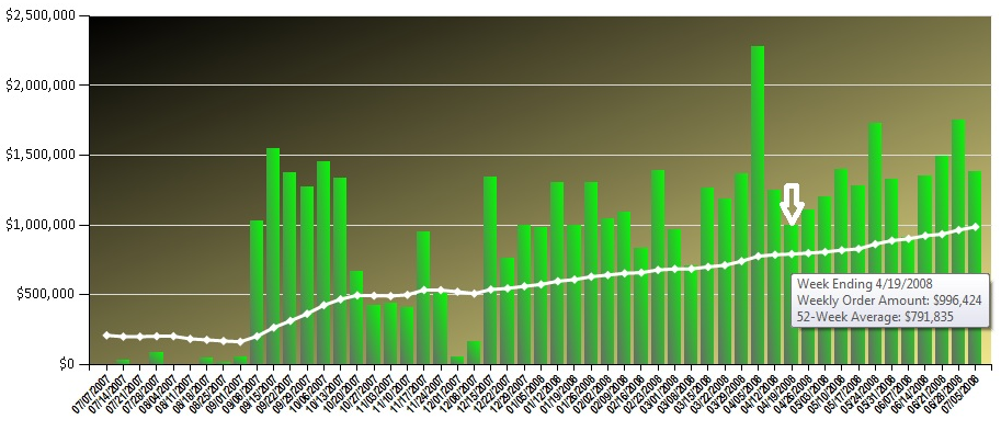
Listings 1 - 3, and Figure 1 demonstrate a result set that summarizes by week-ending date (using a UDF), and also generates a moving average by querying each week against the last 52 weeks - often used for an analytic chart that shows a trend of weeks (Figure 2). The highlights of the T-SQL code are as follows:
First, in order to summarize sales by week, I need a function that will convert any day to a Saturday date, or end of week date (Listing 1). Many developers have probably seen SQL functions that convert dates to Saturday dates - but it’s worth mentioning that when using a date data type, I can’t do the following (which developers have done for years with a datetime data type):
SET @ReturnDate =
 @InputDate +
  (@@DateFirst -
      datepart(weekday,@InputDate
That’s because Microsoft restricted the date data type to only use the DateAdd function: the “+” operator is not valid for the date datatype.
SET @ReturnDate =
  DateAdd(day,
         (@@DateFirst -
            datepart(weekday,@InputDate)),
          @InputDate)
Second, remember that the date range for the result set is the Fiscal Year 2008. Also note that the result set in Figure 1 and the chart in Figure 2 both show all weeks, regardless of whether any purchase orders existed for the week. Many reports/charts need to display all weeks, regardless of whether transactions occurred. Analytically, weeks without data might be as significant as weeks with data. Therefore, a routine (function) that produces all the possible week ending dates will be helpful, especially if many reports need it.
So Listing 2 contains a second function, a table-valued function called CreateDateRange, to create a list of week ending dates for the date range we need. The function uses a recursive query to build a range of dates.
;WITH DateCTE(WeekEndDate) AS
   SELECT @StartDate AS WeekEndDate
      UNION ALL
   SELECT DateAdd(d,7,WeekEndDate)
          AS WeekEndDate
        FROM DateCTE
         WHERE WeekEndDate < @EndDate )
Finally, let’s talk about a calculation involving a 52-week moving average. Essentially, for any one week, we want to get the average sales over the last 52 weeks. For instance, in the tooltip for the plotted point in Figure 2, the week of 4/19/2008 has a 52-week average of roughly $791,835. This means that for the date range of 4/21/2007 to 4/19/2008, the average weekly sales was roughly $791,835. (Subsequently, the 52-week average for the week ending 4/26/2008 would be the average weekly sales from 4/28/2007 to 4/26/2008. This is why we call it a “moving average”, because the range of 52 weeks “moves” with each subsequent week.
Tip 2: Using Table-Valued Functions for Role-based Security
Scenario: I have a SQL query that summarizes purchase orders by Vendor, for a specific ship method. I want our shipping managers to be able to run the query, without actually having SELECT access rights to the table, and so that they can only see summarized vendor orders for their specific ship method.
I frequently go back and forth between OLAP databases and relational databases. I bring this up only because OLAP databases provide dimensional security roles, which make addressing this scenario very easy. However, SQL Server relational databases don’t have built-in row-based security, so we need to implement something.
Because a stated requirement was no SELECT rights to the table, you might be thinking of a stored procedures or a view. Initially this might seem fine, but there are some issues. First, a SQL Server View cannot receive parameters, and we’d need one for the ship method. A stored procedure can certainly receive parameters - and could be a solution - but I’ll add an additional requirement - that database tasks run by a ship manager might want to use the results of the query as an intermediate result set, and subsequently join to other data. Result sets from stored procedures don’t work perfectly in this scenario - you can’t directly join the results of a stored procedure without introducing another table or temp table. Ironically, a view might be better - but we already know that views can’t receive parameters. So what can we do?
A feature in SQL Server 2005 that, to this day, doesn’t get enough attention is table-valued functions. I showed a TVF in Tip #1 to produce a date range - as it turns out, we can use TVFs in this scenario as well.
Listing 4 shows how table-valued functions can be used in conjunction with views to consolidate queries for role-based security. The code walks through creating a TVF with a parameter and then a set of views - and then sets rights for two logins to the views. This helps to overcome a limitation of SQL views - that you can’t pass parameters to them.
Tip 3: SQL Server Covering Indexes
Suppose you’re querying against an invoice table, based on a customer key - and you plan to return non-indexed columns (quantities, dollar amounts, etc.). Even if the query can optimize the customer key, SQL Server still must perform a lookup into the table (or clustered index) to return the other columns.
You can increase performance and lower the number of reads by creating a COVERING INDEX. This type of index will allow you to “bring along other columns for the ride” so that SQL Server won’t have to read into the table or clustered index. In other words, the index covers the entire query.
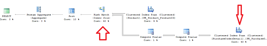
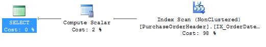
For example, Listing 5 shows a query that sums product line item dollar amounts for specific products - and the query generates an execution plan with an index scan (Figure 3).
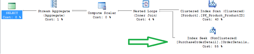
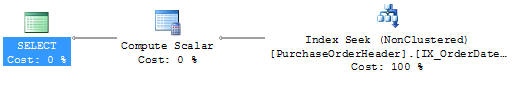
You can optimize the query by creating a non-clustered index that also “covers” the dollar amount. Note the improved execution plan that does an index seek (Figure 4). Also note the STATISTICS IO, and the reduced number of reads when using a covering index.
Covering indexes come at a cost - they increase the size of the index, and might introduce performance issues when rows are add/deleted. So their benefits and costs need to be examined - but there is no question that they can greatly enhance query performance.
Covering indexes….can help with performance, but they’re also larger and might slow down insertions.
Also note that the columns you “include” are not part of the index key itself.
Tip 4: SQL Server SARGs (Searchable Arguments) and Performance
Take a look at Listing 6 - two queries that retrieve orders for March of 2007. Which is faster - the one that uses the YEAR and MONTH function, or the one that queries BETWEEN two dates?
Answer: the latter, hands down. The reason? SQL Server cannot optimize certain functions. These are not considered SARGable (Search Argument-enabled). SQL Server needs to use an index scan (Figure 5) for the YEAR and month function, but can use an index seek (Figure 6) for the BETWEEN statement.
Also, IO Statistics reports that the optimized query does eight times fewer logical reads, and has a much lower execution cost.
From my last Baker’s Dozen issue, I also showed that LIKE is more optimized than SUBSTRING, for the very same reasons.
Tip 5: Using T-SQL SUM OVER to Calculate a % of Total
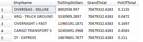
Some people know that we can RANK “over” a set of data, but how many realized that you can do a SUM “over” a set of data? Listing 5 and Figure 7 show how to SUM over a larger set of data, to implement a % of Parent calculation.
This is another example of the “windowing” functions that were introduced in SQL Server 2005, to aggregate/rank “over” a set/window of rows.
Tip 6: Programmatically Disabling SQL Server Constraints and Triggers
In certain data warehousing scenarios, we might want to disable database table constraints and triggers, to optimize performance. Listing 6 shows how we can programmatically disable constraints and triggers, and then re-enable them.
It might seem odd to talk about disabling table constraints. But keep in mind that many ETL scenarios will perform all necessary validations and controls - as if the table constraints didn’t exist to begin with.
Tip 7: Correlated Subqueries vs Derived Table Subqueries
In my last article I talked about a derived table subquery for handling multiple 1-many relationships. In the example, it was impossible to perform all the logic in one SELECT statement, so we needed to pre-aggregate each child table independently.
We can also use correlated subqueries - yes, the much-maligned correlated subquery that, as it turns out, can generate the same execution plan and the same IO Statistics!!!
The much-maligned correlated subquery approach will often generate the same execution plan and IO Statistics. However, a developer should aways check the execution plan and IO Statistics.
Listing 7 shows how we can use correlated subquery expressions to retrieve the summarized purchase order and sales order totals by product. Note that you should ALWAYS view execution plans and IO Statistics before assuming that the database engine will generate a good execution plan for a correlated subquery.
Tip 8: A Brain Teaser on UNION
So you think you know UNION? Maybe you do…or then again….
Did you know that a UNION will perform a duplicate check and a UNION ALL won’t? Did you know you needed an identical number of columns? Did you know that you can only use one ORDER BY, at the end? Did you know that when the UNION performs a duplicate check, it does so across ALL columns?
Listing 8 has a UNION example that appends rows from an employee table and a company table into one result set. See if you can follow along and guess the number of resulting rows at the end. (Sorry, no cash prize if you guess the correct number of rows).
Tip 9: So When Is a Subquery Necessary?
Scenario: I want to see each vendor and their highest order amount - but only if the highest order amount is $150,000 or more.
In my classes where I teach T-SQL programming, a common question is, “How do I know when I NEED a subquery?” To answer this question, we need to understand the data, the SQL language, and also some general patterns.
First, a vendor might have multiple orders that are over $150,000 and are the same order amount (i.e. Vendor 123 might have three orders of $200,000). So we can’t assume that we’ll only be showing one order.
This is a situation where we need to make multiple “dives” into the table…we can’t do it as a single query (you can try, but you won’t succeed!). We need to do the following, as separate steps:
First, we need to determine the highest dollar amount by vendor (for those orders greater than $150,000) and place that into a temporary result set or subquery.
Second, we need to take that list and dive “back” into the table to get the corresponding order IDs for that specific vendor and dollar amount. (Remember, there could be more than one order.)
Listing 11 shows an example where a subquery is needed to first retrieve maximum order amounts by customer, and then turn back around and retrieve the specific orders.
Tip 10: The tinyint data type
There’s no code sample for this one - just a brief discussion about the use of the tinyint datatype in SQL Server. This data type is perfect for status codes and business enumeration values. A tinyint can go from a range of 0-255, and only occupies one byte of storage per value
Tip 11: DISTINCT vs GROUP BY
Suppose we wanted to get a distinct list of names and see how many names are duplicated? Suppose we also wanted to know the number of duplications?
Some developers will use DISTINCT and some will use GROUP BY. Keep in mind that we are talking about two different behaviors. DISTINCT is great to produce a unique list but it won’t tell us if “John Smith” exists five times, if “Mary Wilson” exists four times, etc. For that, we need a GROUP BY with a COUNT aggregation, as well as a HAVING to filter on the number of COUNT aggregations. Listing 12 illustrates the difference between the two statements.
Tip 12: Creating a Result Set of Integers
A while back, a friend of mine was trying to figure out how to write a query to produce a result set of 20 integers (a sequence of numbers from 1-20).
Sure, you can create a variable and use a WHILE but that requires multiple lines of code, and you might be in a situation where the ONLY thing you can write is a SELECT statement.
Yes, you could also do 20 UNION statements. There’s also another way, using the recursive capabilities of a common table expression. Listing 13 shows a query to create a result set of 20 sequences using basic recursion.
Tip 13: INSTEAD OF Triggers for DELETE Scenarios
In some data warehousing scenarios (and even some OLTP databases), DELETE is a four-letter word. Companies might mark rows as inactive, but might not want to DELETE rows.
You might think that if there are PK/FK constraints, then it wouldn’t be possible to DELETE a row that had child transactions. That’s assuming that PK/FK constraints exist….one could argue they SHOULD….but that’s not a given.
So the developer team might implement an inactive status…..but suppose someone isn’t fully aware (but has rights), and tries to manually DELETE a row? Well, what’s needed is a big (and intelligent) watchdog that will sit in front of table/row, stop any deletion attempts and turn them into updates on the inactive status.
Well, SQL Server has such a watchdog - the database trigger - and in this case, an INSTEAD OF trigger. Essentially we can create an INSTEAD OF trigger on a DELETE. This trigger will fire when a process attempts to DELETE a row - and the code in the trigger can update the row’s status flag “instead of” deleting the row. Listing 14 shows an example of an INSTEAD OF trigger on DELETE actions. Note that the trigger code reads the system DELETED table to capture the rows that the application/user tried to delete - and instead, updates the rows with an inactive status.
Next Time Around in the Baker’s Dozen
In my next article, I’ll talk about some of the great new features in SQL Server 2012 (“Denali”). SQL Server 2012 has a new Column Store index that can greatly help the performance of certain data warehousing queries, several new T-SQL features, new and improved functionality in SSIS, and an entirely new landscape for creating business intelligence applications. Stay tuned!