


Very often, when people talk about data analytics, Pandas is the first library that comes to mind. And, of course, in more recent times, Polars is fast gaining traction as a much faster and more efficient DataFrame library. Despite the popularity of these libraries, SQL (Structured Query Language) remains the language that most developers are familiar with. If your data is stored in SQL-supported databases, SQL is one of the easiest and most natural ways for you to retrieve your data.
Recently, with Python becoming the lingua franca of data science, most attention has shifted to techniques on how to manipulate data in tabular format (most notably stored as a DataFrame object). However, the real lingua franca of data is actually SQL. And because most developers are familiar with SQL, isn't it more convenient to manipulate data using SQL? This is where DuckDB comes in.
In this article, I'll explain what DuckDB is, why it's useful, and, more importantly, I want to walk you through examples to demonstrate how you can use DuckDB for your data analytics tasks.
What Is DuckDB?
DuckDB is a Relational Database Management System (RDBMS) that supports the Structured Query Language (SQL). It's designed to support Online Analytical Processing (OLAP), and is well suited for performing data analytics. DuckDB was created by Hannes Muehleisen and Mark Raasveldt, and the first version released in 2019.
Unlike traditional database systems where you need to install them, DuckDB requires no installation and works in-process. Because of this, DuckDB can run queries directly on Pandas data without needing to import or copy any data. Moreover, DuckDB uses vectorized data processing, which makes it very efficient - internally, the data is stored in columnar format rather than row-format (which is commonly used by databases systems such as MySQL and SQLite).
Think of DuckDB as the analytical execution engine that allows you to run SQL queries directly on existing datasets such as Pandas DataFrames, CSV files, and traditional databases such as MySQL and Postgres. You can focus on using SQL queries to extract the data you want.
Why DuckDB?
Today, your dataset probably comes from one or more of the following sources:
- CSV files
- Excel spreadsheets
- XML files
- JSON files
- Databases
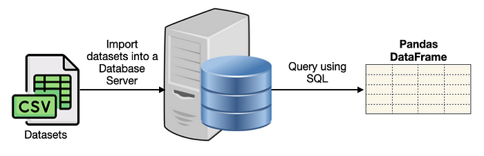
If you want to use SQL to manipulate your data, the typical scenario is to first load the dataset (such as a CSV file) into a database server. You then load the data into a Pandas DataFrame through an application (such as Python) using SQL (see Figure 1).
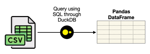
DuckDB eliminates the need to load the dataset into a database server and allows you to directly load the dataset using SQL (see Figure 2).
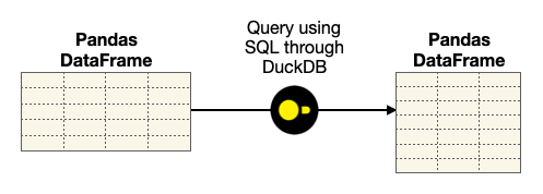
Once the DataFrame is loaded, you can use DuckDB and SQL to further slice and dice the DataFrame (see Figure 3).
Data Analytics Using the Insurance Dataset
The best way to understand DuckDB is through examples. For this, I'll use the insurance dataset located at https://www.kaggle.com/datasets/teertha/ushealthinsurancedataset?resource=download. The insurance dataset contains 1338 rows of insured data, where the insurance charges are given against the following attributes of the insured: age, sex, BMI, number of children, smoker, and region. The attributes are a mix of numeric and categorical variables.
Loading the CSV File into Pandas DataFrames
Let's examine the insurance dataset by loading the insurance.csv file into a Pandas DataFrame:
import pandas as pd

df_insurance = pd.read_csv("insurance.csv")
display(df_insurance)
Figure 4 shows how the DataFrame looks.
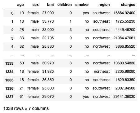
The various columns in the DataFrame contain the various attributes of the insurance customer. In particular, the charges column indicates the individual medical costs billed by health insurance (payable by the insured).
Creating a DuckDB Database
Before you can create a DuckDB database, you need to install the duckdb package using the following command:
!pip install duckdb
To create a DuckDB database, use the connect() function from the duckdb package to create a connection (a duckdb.DuckDBPyConnection object) to a DuckDB database:
import duckdb
conn = duckdb.connect()
You can then register the DataFrame that you loaded earlier with the DuckDB database:
conn.register("insurance", df_insurance)
The register() function registers the specified DataFrame object (df_insurance) as a virtual table (insurance) within the DuckDB database.
Directly Loading the CSV into a Pandas DataFrame Using DuckDB
Instead of loading a DataFrame manually and then registering with the DuckDB database, you can also use the connection object to read a CSV file directly, like this:
conn = duckdb.connect()

df = conn.execute('''
    SELECT
      *
    FROM read_csv_auto('insurance.csv')
''').df()

conn.register("insurance", df)
In the above code snippet:
- I used a SQL statement with the
read_csv_auto()function to read a CSV file. Theexecute()function takes in this SQL statement and executes it. - The
df()function converts the result of theexecute()function into a Pandas DataFrame object. - Once the DataFrame is obtained, use the
register()function to register it with the DuckDB database.
You can confirm the number of tables in the DuckDB by using the SHOW TABLES SQL statement:
display(conn.execute('SHOW TABLES').df())
The result is shown in Figure 5.
To fetch rows from the insurance table, you can directly use a SQL statement using the execute() function:
df = conn.execute(
         "SELECT * FROM insurance").df()
df
The output will be the same as shown earlier in Figure 4.
Performing Analytics Using DuckDB
Let's now perform some useful data analytics using the insurance table in the DuckDB. First, I want to visualize the distribution of charges based on sex:
import seaborn as sns
import matplotlib.pyplot as plt
f, ax = plt.subplots(1, 1, figsize=(5, 3))
df = conn.execute('''
    SELECT
        *
    FROM insurance
''').df()

ax = sns.barplot(x = 'region',
                 y = 'charges',
                 hue = 'sex',
                 data = df,
                 palette = 'cool',
                 errorbar = None)
The above code snippet uses the Seaborn package to plot a bar plot that shows the various insurance charges for each gender in each of the four regions (see Figure 6 for the output).
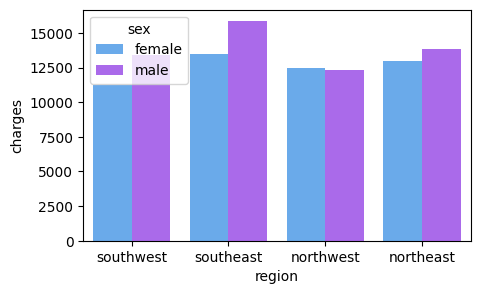
Overall, men tend to have higher medical insurance cost for all regions, except the northwest region.
I'm also interested in visualizing the distribution of insurance charges for people based in the southwest region, based on the number of children a person has. I can do the following:
import seaborn as sns
import matplotlib.pyplot as plt
f, ax = plt.subplots(1, 1, figsize=(7, 5))
df = conn.execute('''
    SELECT
        *
    FROM insurance
    WHERE region = 'southwest'
''').df()

ax = sns.barplot(x = 'region',
                 y = 'charges',
                 hue = 'children',
                 data = df,
                 palette = 'Set1',
                 errorbar = None)
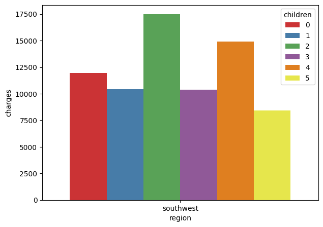
As you can see from Figure 7, for the southwest region, the mean insurance charges for a person with two children is close to $17,500, which is the highest. The lowest mean insurance charges are for people with five children.
Based on the value in the DataFrame df (which contains all the people in the southwest), you can plot linear models to examine the relationships between the various attributes (such as age, bmi, smoker, children) against the insurance charges:
ax = sns.lmplot(x = 'age',
                y = 'charges',
                data = df,
                hue = 'smoker',
                palette = 'Set1')
ax = sns.lmplot(x = 'bmi',
                y = 'charges',
                data = df,
                hue = 'smoker',
                palette = 'Set2')
ax = sns.lmplot(x = 'children',
                y = 'charges',
                data = df,
                hue = 'smoker',
                palette = 'Set3')
Figure 8 shows how the insurance charges relates to age, bmi, and number of children, and whether they are smokers or not.
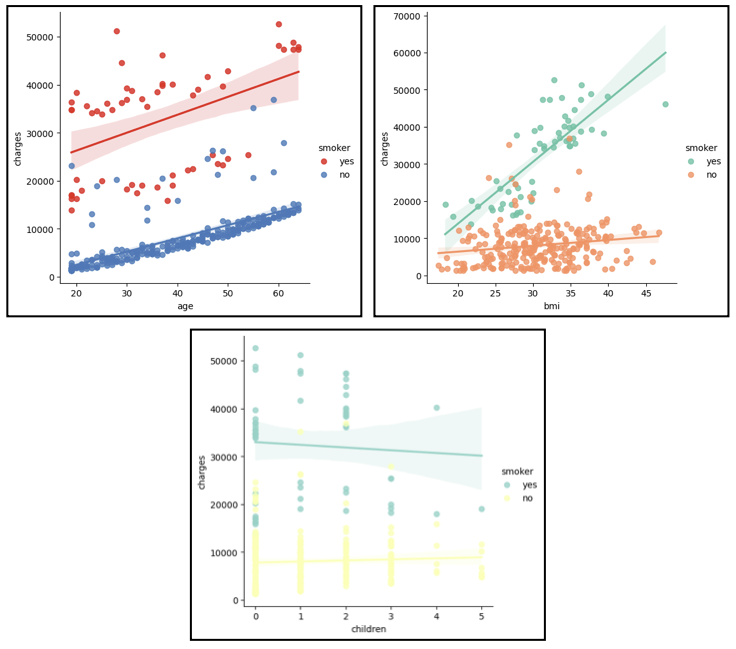
Generally, smokers have to pay much higher insurance charges compared to non-smokers. In the case of smokers, as the age or BMI increases, the amount of insurance charges increases proportionally. The number of children a customer has does not really affect the insurance charges.
Next, I want to visualize the mean insurance charges for all the people in the southeast and southwest regions, so I modify my SQL statement and plot a bar plot:
df = conn.execute('''
    SELECT
        region,
        mean(charges) as charges
    FROM insurance
    WHERE region = 'southwest' or
          region = 'southeast'
    GROUP BY region
''').df()

f, ax = plt.subplots(1, 1, figsize=(5, 3))
ax = sns.barplot(x = 'region',
                 y = 'charges',
                 data = df,
                 palette = 'Reds')
Figure 9 shows the plot.
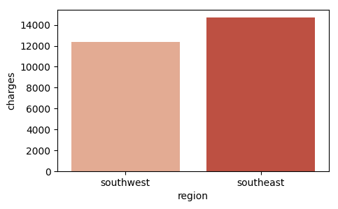
Overall, the insurance charges are higher for people in the southeast region than those in the southwest region.
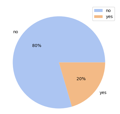
Next, I want to see the proportion of smokers for the entire dataset:
palette_color = \ seaborn.color_palette('pastel')
plt.figure(figsize = (5, 5))

df = conn.execute('''
    SELECT
        count(*) as Count, smoker
    FROM insurance
    GROUP BY smoker
    ORDER BY Count DESC
''').df()

plt.pie('Count',
        labels = 'smoker',
        colors = palette_color,
        data = df,
        autopct='%.0f%%',)

plt.legend(df['smoker'], loc="best")
The pie chart in Figure 10 shows the proportion of smokers (20%) vs. non-smokers (80%).
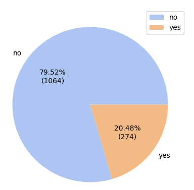
It would be more useful to be able to display the numbers of smokers and non-smokers alongside their percentages. So let's add a function named fmt() to customize the labels displayed on each pie on the pie chart:
# sum up total number of people
total = df['Count'].sum()
def fmt (x):
    # display percentage followed by number
    return '{:.2f}%\n({:.0f})'.format(x, total * x / 100)

palette_color = \ seaborn.color_palette('pastel')
plt.figure(figsize = (5, 5))

plt.pie('Count',
        labels = 'smoker',
        colors = palette_color,
        data = df,
        autopct = fmt)  # call fmt()
plt.legend(df['smoker'], loc="best")
Figure 11 shows the updated pie chart.
JSON Ingestion
One of the new features announced in the recent DuckDB release (version 0.7) is the support for JSON Ingestion. Basically, this means that you can now directly load JSON files into your DuckDB databases. In this section, I'll show you how to use this new feature by showing you some examples.
For the first example, suppose you have a JSON file named json0.json with the following content:
[
  {
    "id": 1,
    "name": "Abigail",
    "address": "711-2880 Nulla St.
               Mankato
               Mississippi 96522"
  },
  {
    "id": 2,
    "name": "Diana",
    "address": "P.O. Box 283
                8562 Fusce Rd. Frederick
                Nebraska 20620"
  },
  {
    "id": 3,
    "name": "Jason",
    "address": "606-3727 Ullamcorper. Street
                Roseville
                NH 11523"
  }
]
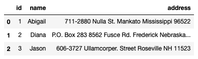
This JSON file contains an array of objects, with each object containing three key/value pairs. This is a very simple JSON file and the easiest way to read it into DuckDB is to use the read_json_auto() function:
import duckdb
conn = duckdb.connect()

conn.execute('''
    SELECT
        *
    FROM read_json_auto('json0.json')
''').df()
The output of the above code snippet is as shown in Figure 12.
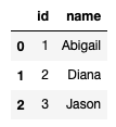
If you only want the id and name fields, modify the SQL statement as follows:
import duckdb
conn = duckdb.connect()

conn.execute('''
    SELECT
        id, name
    FROM read_json_auto('json0.json')
''').df()
You'll now only get the id and name columns (see Figure 13)
The read_json_auto() function automatically reads the entire JSON file into DuckDB. If you only want to selectively read specific keys in the JSON file, use the read_json() function and specify the json_format and columns attributes as follows:
import duckdb
conn = duckdb.connect()

conn.execute('''
    SELECT
        *
    FROM read_json('json0.json',
    json_format = 'array_of_records',
    columns = {
        id:'INTEGER',
        name:'STRING'
    })
''').df()
The output is the same as shown in Figure 13.
Suppose now the content of json0.json is slightly changed and now saved in another file named json1.json:
[
  {
    "id": 1,
    "name": "Abigail",
    "address": {
      "line1":"711-2880 Nulla St.
               Mankato",
      "state":"Mississippi",
      "zip":96522
    }
  },
  {
    "id": 2,
    "name": "Diana",
    "address": {
      "line1":"P.O. Box 283 8562",
      "line2":"Fusce Rd. Frederick",
      "state":"Nebraska",
      "zip":20620
    }
  },
  {
    "id": 3,
    "name": "Jason",
    "address": {
      "line1": "606-3727 Ullamcorper",
      "line2":"Street Roseville",
      "state":"NH",
      "zip": 11523
    }
  }
]
As you can see, the address of each person is now split into four different key/value pairs: line1, line2, state, and zip. Notice that the first person does not have a line2 attribute in its address.
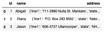
As usual, you can use the read_json_auto() function to read the JSON file:
import duckdb
conn = duckdb.connect()

conn.execute('''
    SELECT
        *
    FROM read_json_auto('json1.json')
''').df()
Observe that the address field is now a string containing all the four key/value pairs (see Figure 14).
So how do you extract the key value pairs of the addresses as individual columns? Fortunately you can do so via the SQL statement:
import duckdb
conn = duckdb.connect()

conn.execute('''
    SELECT
        id,
        name,
        address['line1'] as line1,
        address['line2'] as line2,
        address['state'] as state,
        address['zip'] as zip,
    FROM read_json_auto('json1.json')
''').df()
Figure 15 now shows the key/value pairs for the addresses extracted as individual columns.
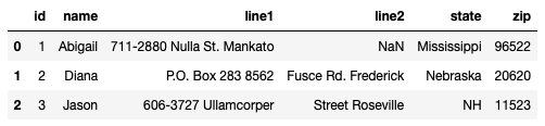
As the first person doesn't have the line2 attribute, it has a NaN value in the DataFrame.
Consider another example (json2.json) where all the information you've seen in the previous examples are encapsulated within the people key:
{
  "people": [
    {
      "id": 1,
      "name": "Abigail",
      "address": {
        "line1":"711-2880 Nulla St. Mankato",
        "state":"Mississippi",
        "zip":96522
      }
    },
    {
      "id": 2,
      "name": "Diana",
      "address": {
        "line1":"P.O. Box 283 8562 ",
        "line2":"Fusce Rd. Frederick",
        "state":"Nebraska",
        "zip":20620
      }
    },
    {
      "id": 3,
      "name": "Jason",
      "address": {
        "line1": "606-3727 Ullamcorper",
        "line2":"Street Roseville",
        "state":"NH",
        "zip": 11523
      }
    }
  ]
}
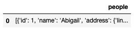
If you try to load it using read_json_auto(), the people key will be read as a single column (see Figure 16).
import duckdb
conn = duckdb.connect()
import json

conn.execute('''
    SELECT
        *
    FROM read_json_auto('json2.json')
''').df()
To properly read it into a Pandas DataFrame, you can use the unnest() function in SQL:
import duckdb
conn = duckdb.connect()
import json

conn.execute('''
    SELECT
        p.id,
        p.name,
        p.address['line1'] as line1,
        p.address['line2'] as line2,
        p.address['state'] as state,
        p.address['zip'] as zip,
    FROM (
              SELECT unnest(people) p
              FROM read_json_auto('json2.json')
          )
''').df()
The JSON file is now loaded correctly, just like Figure 15.
Summary
If you're a hardcore SQL developer, using DuckDB is a godsend when performing data analytics. Instead of manipulating DataFrames, you could now use your SQL knowledge to manipulate the data in whatever form you want. Of course, you still need a good working knowledge of DataFrames, but the bulk of the analytics part can be performed using SQL. In addition, JSON support in the latest version of DuckDB is definitely useful. Even so, loading the JSON properly into the required shape definitely takes some getting used to. Things are still rapidly evolving and hopefully, the next version will make things even easier!